Welcome to the tutorial section of our web server, where we aim to provide you with a detailed guide on our Analysis function. Following your data preparation and data uploading, we offer two distinct options for analysis:
A Step-to-Step
process for those who
prefer a more
hands-on approach, and
A One-Click
process
for efficiency and
convenience.
Each option is accompanied by comprehensive tutorials to assist you every step of the way.
Microbial Profile Requirement:
Implementation of xMarkerFinder requires pre-processed microbial profiles from at least three cohorts (here a cohort is defined as dataset from an individual study). Taxonomic, functional, and genetic variation profiles derived from amplicon sequencing and whole-genome sequencing are all allowed.
We encourage the re-use and exploration of public datasets, as well as generating new microbiome datasets via processing sequencing data with consistent pipelines to reduce technical heterogeneity.
To assist researchers in identifying suitable datasets more effectively for their own research endeavors, we have integrated metadata of publicly available microbiome datasets from several curated sources in our Resource Page.
Metadata Requirement:
To better account for inter-cohort and inter-individual differences and correct for confounding effects,detailed metadata information is encouraged, including but not limited to demographic and biogeographic variables, such as Age, BMI, and sex.
Dataset Requirement:
To ensure comprehensive analyses, we require three sets of microbial abundance profiles and corresponding metadata: training dataset, test dataset, and non-target datasets.
Training dataset and test dataset: We recommend users to split their input microbial profiles into a training set and an external test set. xMarkerFinder mandates at least three cohorts within the training set to bolster biomarker robustness and ensure extensive internal validations. Users can designate specific cohorts as training or test datasets. Alternatively, they can also sample a proportion (20%-40% as recommended) from each cohort of the training dataset to serve as the test dataset.
Non-target datasets: Given the broad impact of microbial imbalances across various diseases and scenarios, it's crucial that our biomarkers maintain a high degree of specificity. Here, to mitigate false positives in both clinical and environmental contexts, we also require microbial profiles from non-target datasets (datasets of different diseases/exposures/environmental scenarios beyond the training and test datasets), accompanied by relevant metadata. This approach allows us to simulate the examination of biomarkers in a prospective setting using retrospective data, providing sufficient evidence for biomarker identification and validation.
Submit data:
Users can freely upload their datasets for analysis. We have provided Must-Read Tips to assist with the upload process. It’s mandatory to upload both the training and test datasets, along with their respective metadata. Additionally, if non-target datasets are available, users can upload them for specificity assessment and complete the whole workflow of xMarkerFinder.
Just upload all the datasets and hit the Submit button!

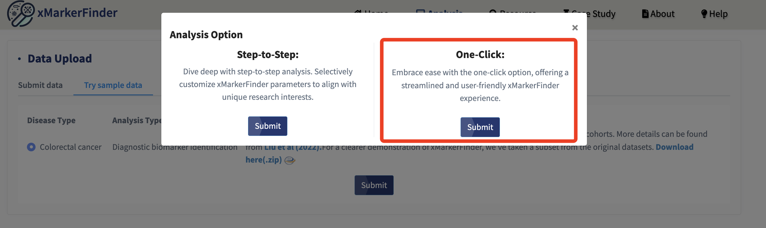
Try sample data:
Alternatively, we provide sample datasets from our prior research publication, featuring metagenome data of colorectal cancer (CRC) patients and healthy controls from seven cohorts. For a clearer demonstration of xMarkerFinder, we've selected a subset from the original datasets.
Just click the Submit button!
Six example files are displayed, making it straightforward for users to grasp the specific purpose of each data file. Click Confirm!
Once data is uploaded, we offer two modes of analysis: Step-by-Step and One-Click.

Data preprocessing:
Data normalization: To mitigate challenges induced by different number of sequencing (e.g., library size), microbial count matrices are often normalized by various computational strategies prior to downstream analyses. Here, xMarkerFinder introduces various normalization methods, including proportional relative abundance (REL, as default), arcsine square root (AST), centered log-ratio (CLR), and trimmed mean of m-values (TMM).
REL: REL calculates the relative abundance of each feature in every sample, giving the count/total count of each feature.
AST: AST calculates the arcsine square root transformation based on normalized relative abundance.
CLR: CLR transforms all features within each sample into a log scale, calculates the geometric mean of all features, and centralizes on this basis.
TMM: TMM takes the logarithm of the original count matrix to obtain M-values, fits the cumulative density distribution function of the M values of each sample, crops off the two ends, obtains the average value of the core interval as trimmed value, and calculates the M value of each sample / trimmed value of the sample.
Users can choose one of these methods and click the Submit button. All abundance files will be normalized for subsequent analyses.
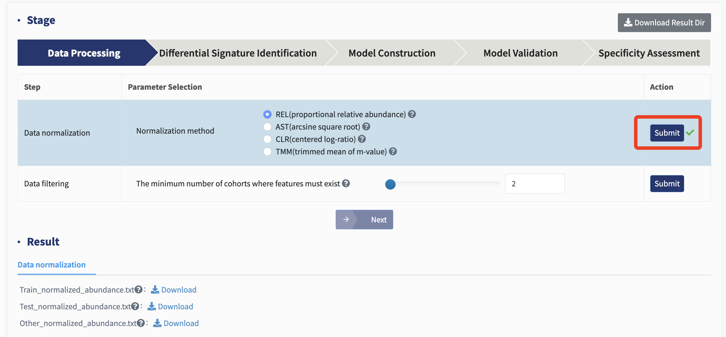
Data filtering: Infrequent signatures, those with low occurrence rates across cohorts are discarded (default: prevalence below 20% of samples from a given cohort) to ensure that identified biomarkers are reproducible and could be applied to prospective cohorts.
Users can select the minimum number of cohorts where features must exist and click Submit: . The number of feature post-filtering will be displayed.

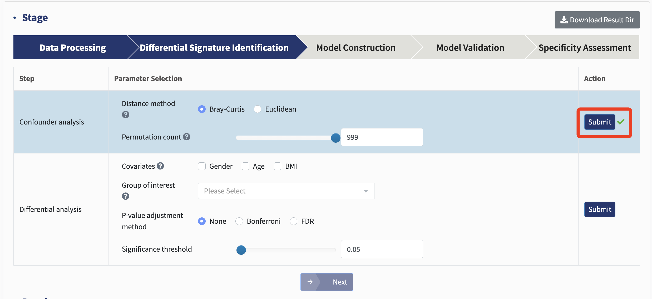
Differential signature identification:
Confounder analysis: Inter-cohort heterogeneity caused by variance in confounders is inevitable in meta-analyses, strongly affecting downstream differential signature identification. Permutational multivariate analysis of variance (PERMANOVA) test quantifies microbial variations attributable to each metadata variable, thus assigning a delegate to evaluate confounding effects. PERMANOVA test here is performed on Bray-Curtis and Euclidean matrices. For REL and TMM normalization method, please select Bray-Curtis distance. For AST and CLR normalization method, Euclidean distance is recommended.
Click Submit and start the analysis!
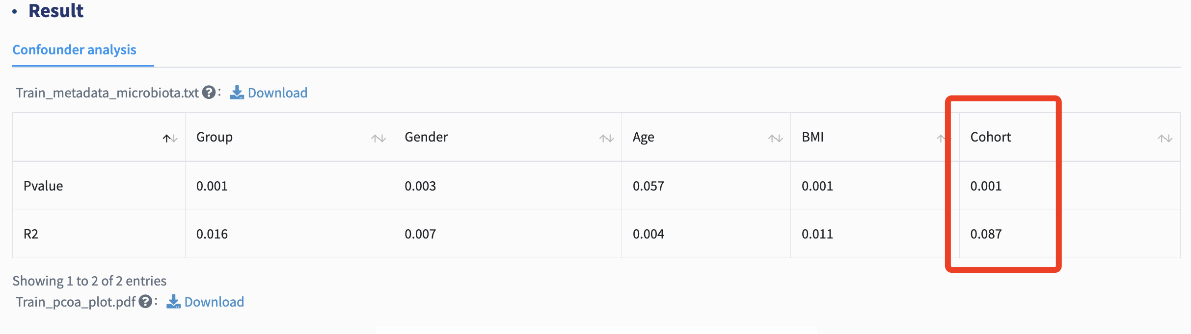
For each metadata variable, coefficient of determination (R2) value and p value are calculated to explain how variation is attributed. The variable with the most predominant impact on microbial profiles is treated as major batch, and other confounders are subsequently used as covariates in the following differential analysis.
Differential analysis: To identify disease or trait-associated microbial signatures across cohorts, MMUPHin is employed. Regression analyses in individual cohorts are performed, where multivariable associations between phenotypes, exposures, experimental groups or other metadata factors and microbial profiles are determined. These results are then aggregated with established fixed effects models to test for consistently differential signatures between groups.
In the differential analysis, the batch refers to the Cohort in the metadata. Other important metadata factors,identified through confounder analysis to significantly influence microbial profiles ( p value <0.05), are used as covariates, such as Age, Gender, and BMI.
Simply choose the covariates from your own data and the desired Group of interest (such as a disease group, exposed group, or deep water) and hit Submit! Users can also choose whether or not to adjust the p values and the adjustment method.
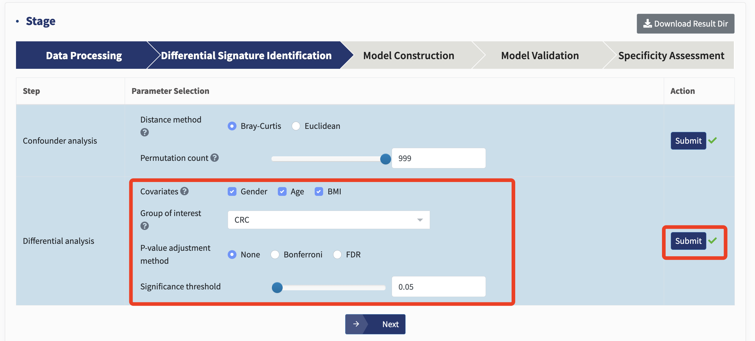
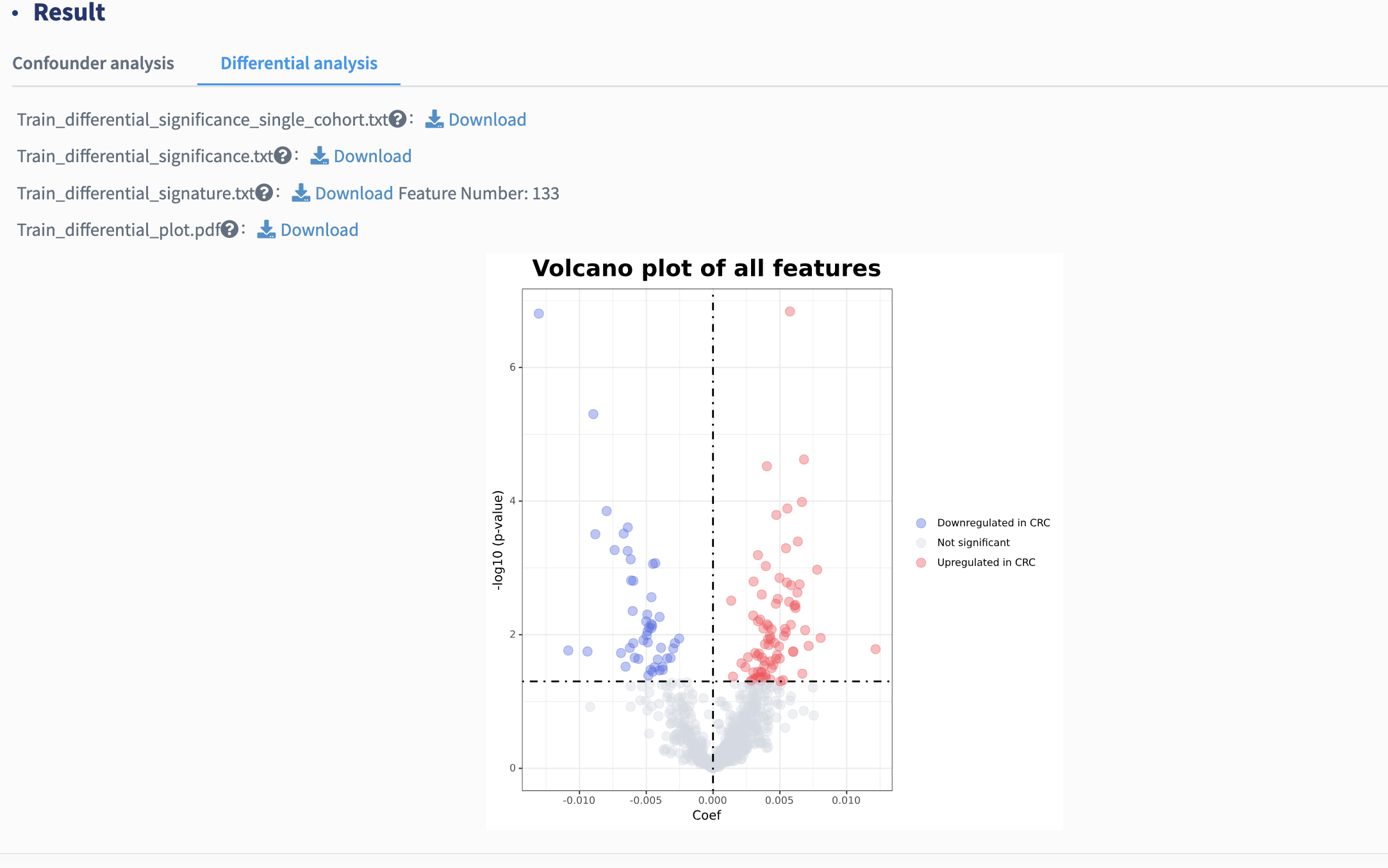
Signatures with consistently significant differences in meta-analysis (default p values less than 0.05) are identified as cross-cohort differential signatures and used for further feature selection in subsequent stages. Here, a volcano plot showing the differential signatures is provided. Each point represents a feature. Coefficient > 0, P < .05 (in red): features significantly more abundant in group of interest compared with control; Coefficient < 0, P < .05 (in blue): features significantly less abundant in group of interest compared with control; P > .05 (in gray): non-differential features.
Model construction
Classifier selection: xMarkerFinder integrates multiple widely used ML algorithms, including Logistic Regression (LR, L1 and L2 regularization), Support Vector classifier (SVC) with the Radial Basis Function kernel, K-nearest Neighbors (KNN) classifier, Decision Tree (DT) classifier, Random Forest (RF) classifier, and Gradient Boosting (GB) classifier.
Just click Submit to conduct the classifier selection!
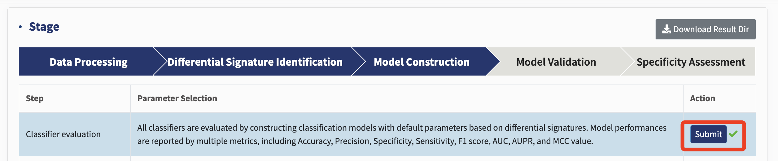
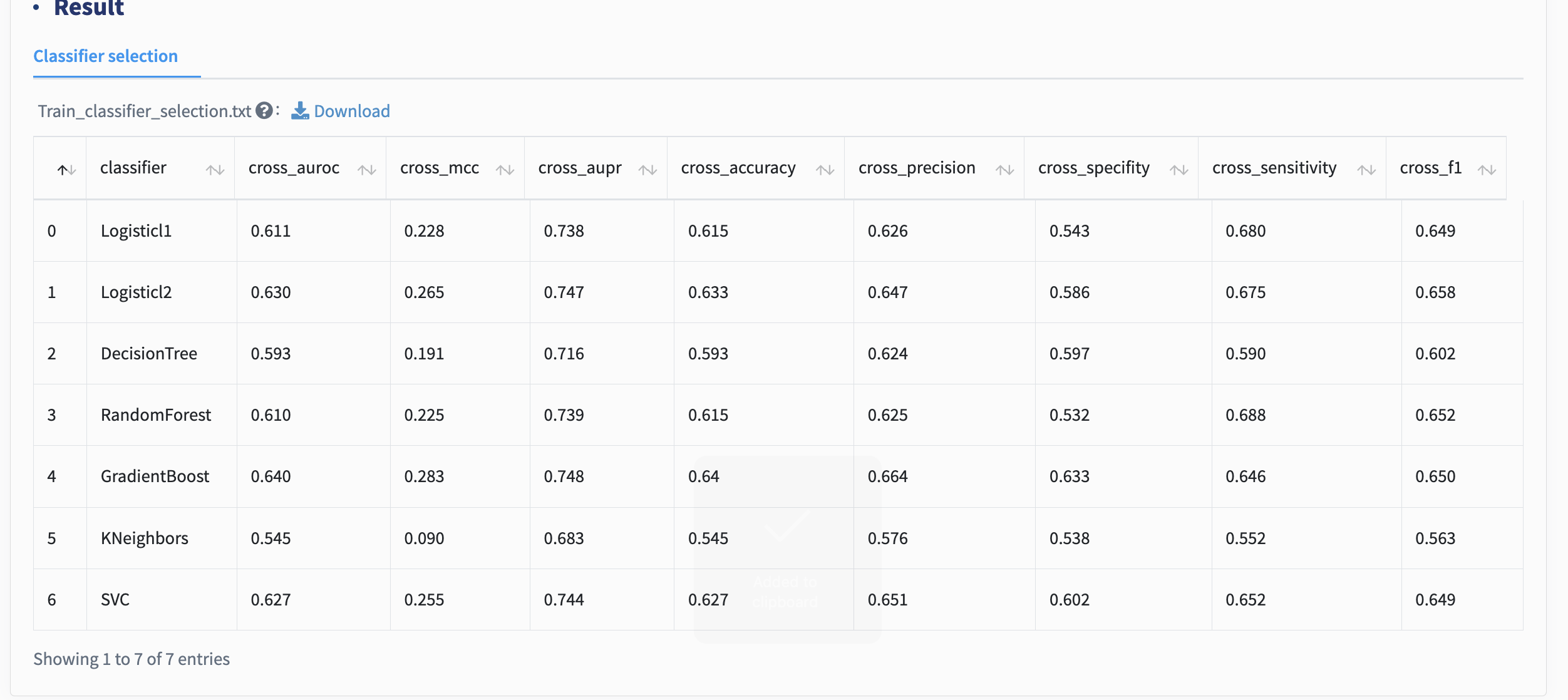
All classifiers are assessed by constructing classification models with default parameters based on differential signatures. Throughout this whole workflow, multiple model evaluation metrics are used to evaluate model performances (Table 1). Despite various ML algorithms provided in xMarkerFinder, RF has been shown to outperform, on average, other learning tools for microbiome data, and is recommended as the default classifier. When selecting a model, we recommend focusing primarily on AUC, AUPR, and MCC, while using other metrics as supplementary indicators for decision-making.
| Metric | Computation | Meaning |
|---|---|---|
| Accuracy | (TP+TN)/(TP+FP+FN+TN) | Ratio of correct predictions to total predictions. |
| Precision | TP/(TP+FP) | Ratio of TPs to total predicted positives. |
| Specificity | TN/(TN+FP) | Ratio of TNs to total negatives. |
| Sensitivity | TP/(TP+FN) | Ratio of TPs to total positives. |
| F1 score | 2*(Sensitivity*Precision) /(Sensitivity+Precision) | F1 score considers both precision and sensitivity, and calculates the harmonic mean of them. |
| AUC | The area under the receiver operating characteristic (ROC) curve (the plot of the Sensitivity as y-axis versus 1-Specificity as x-axis). | A summary of the model performance, representing its discriminative power. |
| AUPR | The area under the precision-recall curve | AUPR summarizes the precision-recall tradeoff. |
| MCC | (TP x TN - FP x FN) / sqrt((TP + FP) * (TP + FN) * (TN + FP) * (TN + FN)) | MCC provides a balanced measure ranging from -1 to 1, with 1 being the perfect model. |
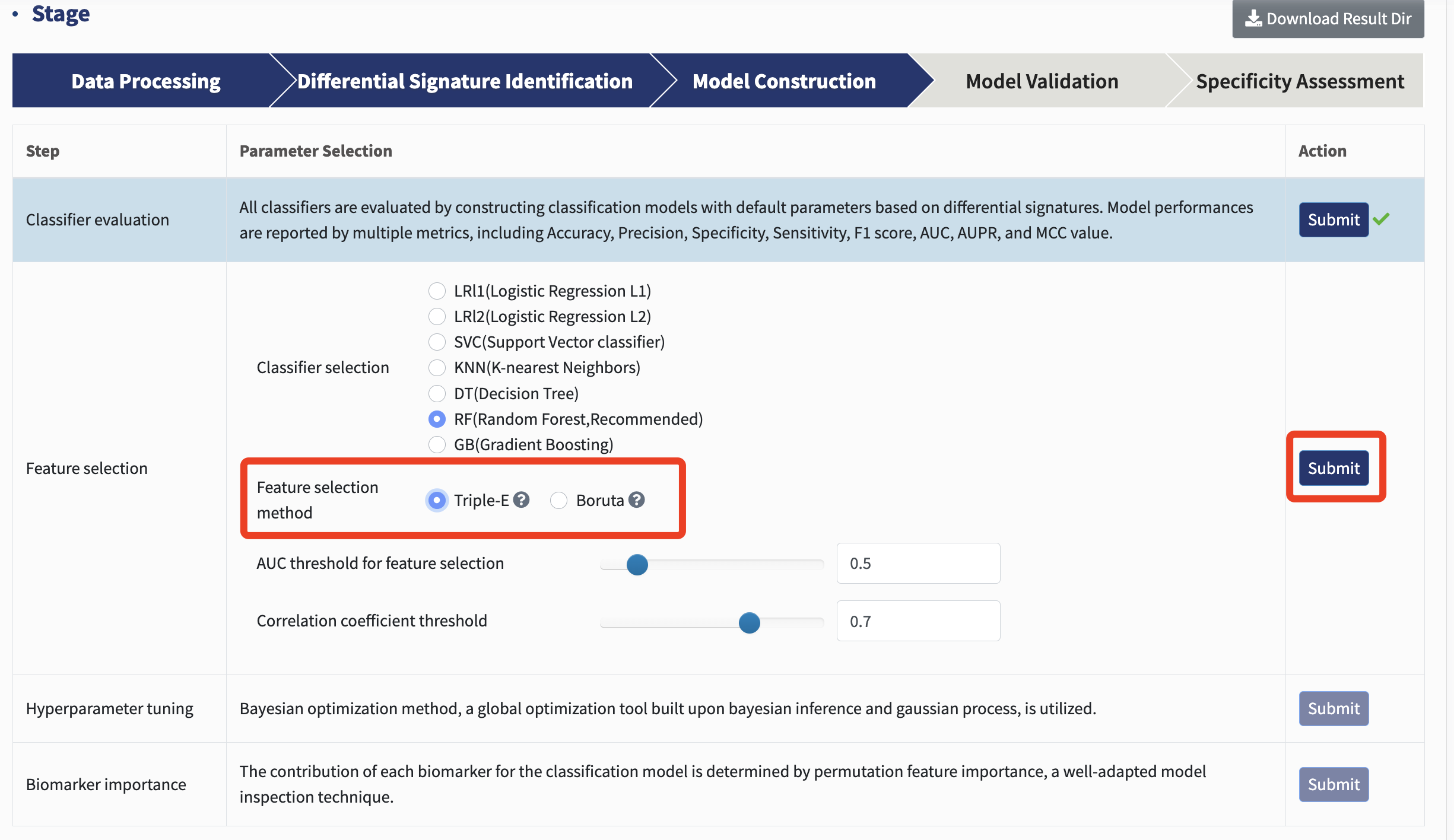
Feature selection: xMarkerFinder offers users a choice between two distinct feature selection methods. One of the highlights is the Triple-E feature selection procedure, designed to pinpoint an optimal panel of candidate biomarkers.
The first step, “feature effectiveness evaluation,” selects features based on their discriminative power. Specifically, each differential signature is used to construct a classification model with default parameters. Signatures with AUC values exceeding 0.5 (by default) are deemed predictive and retained as effective features.
The second step, “collinear feature exclusion,” is crafted to sidestep collinearity by omitting features that are highly correlated, retaining only uncorrelated-effective features, with a threshold of Spearman’s rank correlation coefficient greater than 0.7 as a default.
The last step of Triple-E process is the “recursive feature elimination”, which determines the optimal panel of features with the highest predictive potential, earmarking them as candidate biomarkers.
Users can select the AUC and correlation coefficient threshold for Triple-E feature selection and hit Submit. If you're unsure about which parameters to select, we recommend using our default settings.
Additionally, xMarkerFinder introduces the Boruta feature selection as an alternative. In this method, “shadow features” are produced by randomly shuffling copies of all original features. During each iteration, these shadow features are combined with the original ones to train a classifier, from which feature importances are derived. Original features deemed less significant than any shadow feature are considered unimportant and excluded from the subsequent iteration. The process concludes when all features are classified as either important or unimportant, with only the important features retained as candidate biomarkers.
For Boruta feature selection, users can choose from using the differential signatures generated by differential analysis or effective features / uncorrelated-effective features produced by Triple-E. Just select and click Submit!
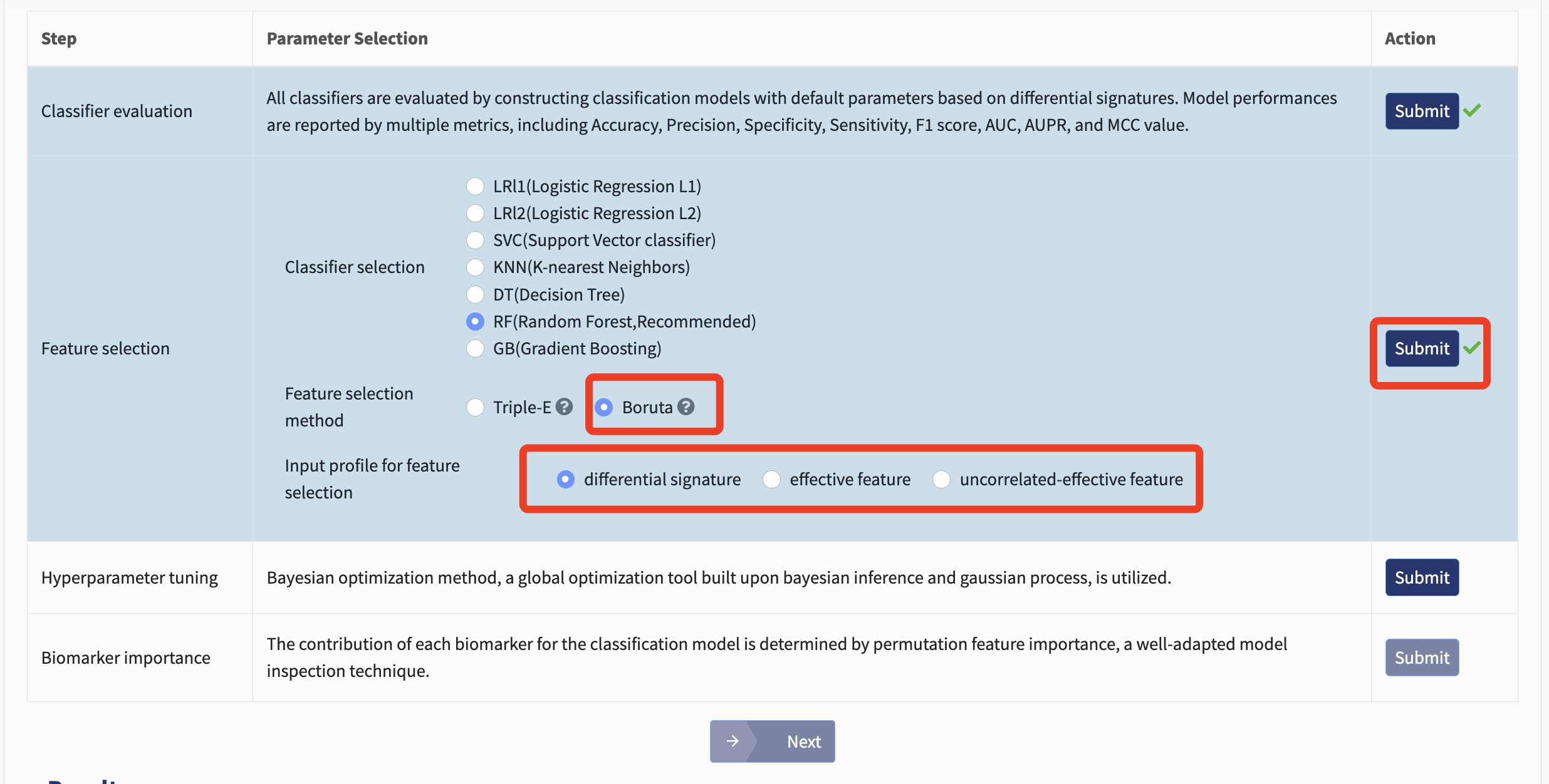
Both feature selection methods will produce a collection of candidate biomarkers for model construction and validation.
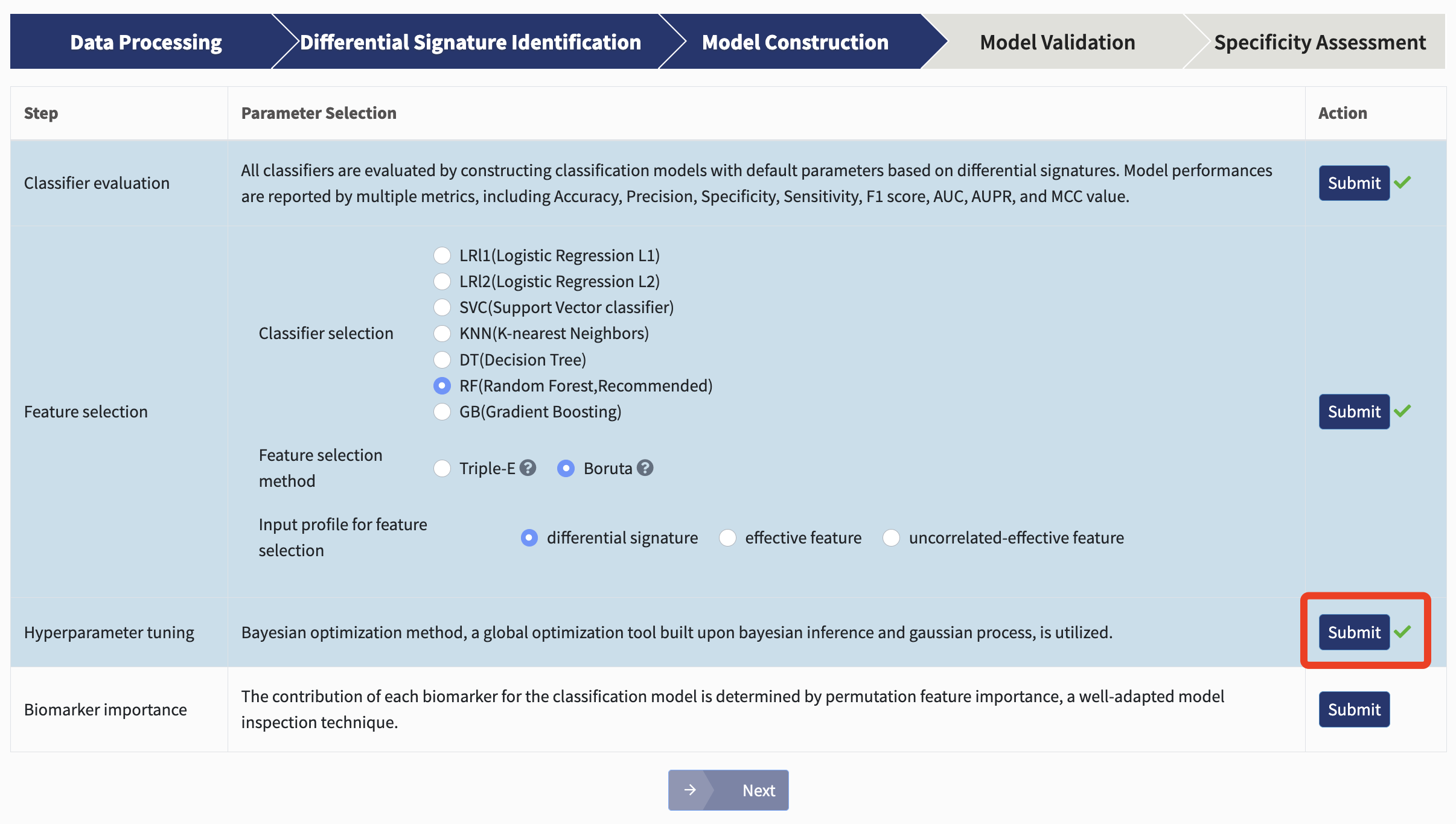
Hyperparameter tuning: Based on the selected classifier, candidate biomarkers are used to construct a classification model with stratified five-fold cross-validation to exhibit their predictive abilities, the hyperparameters of which are tuned via bayesian optimization method, a global optimization tool built upon bayesian inference and gaussian process.
Just hit Submit!
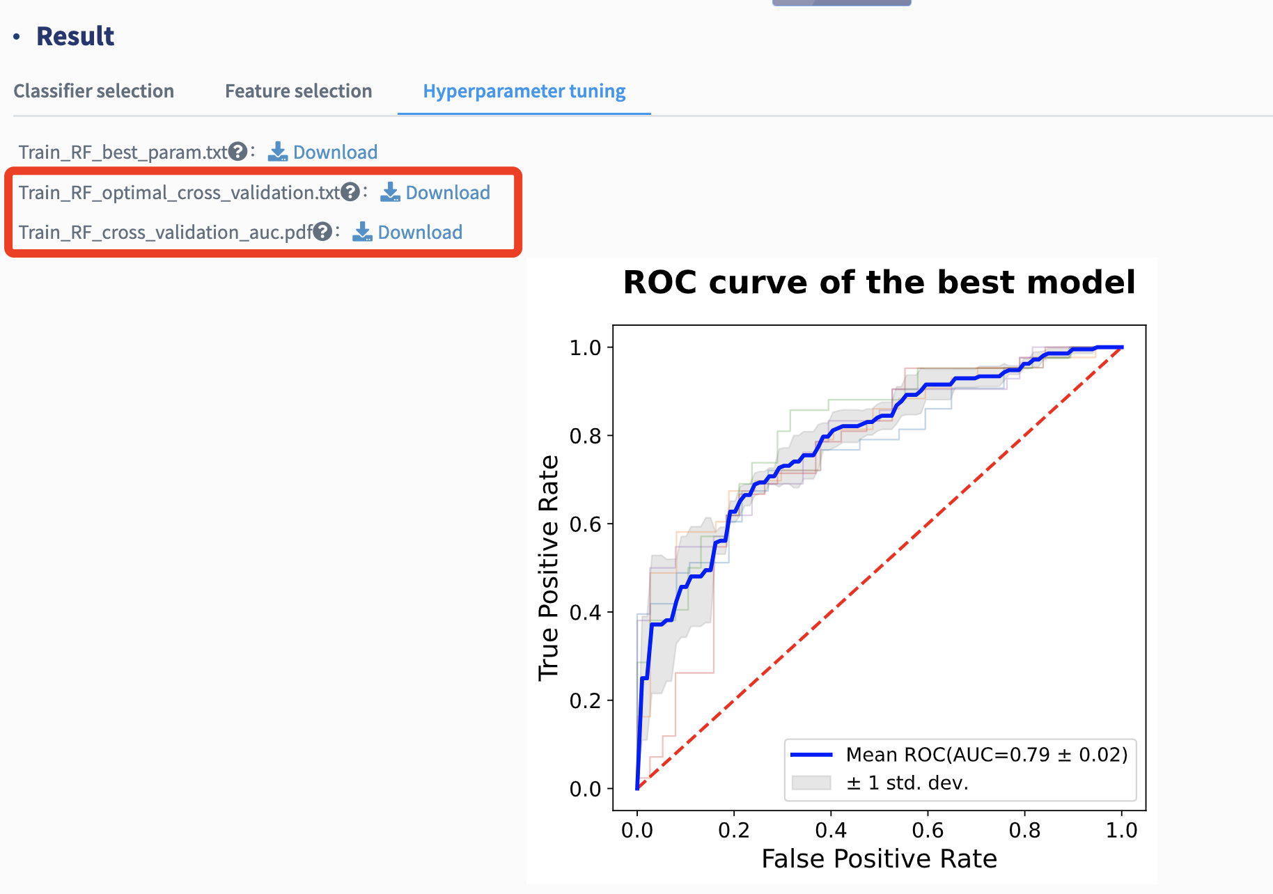
The general performance of the best-performing model is reported with several metrics mentioned above and its cross-validation AUC plot is provided.
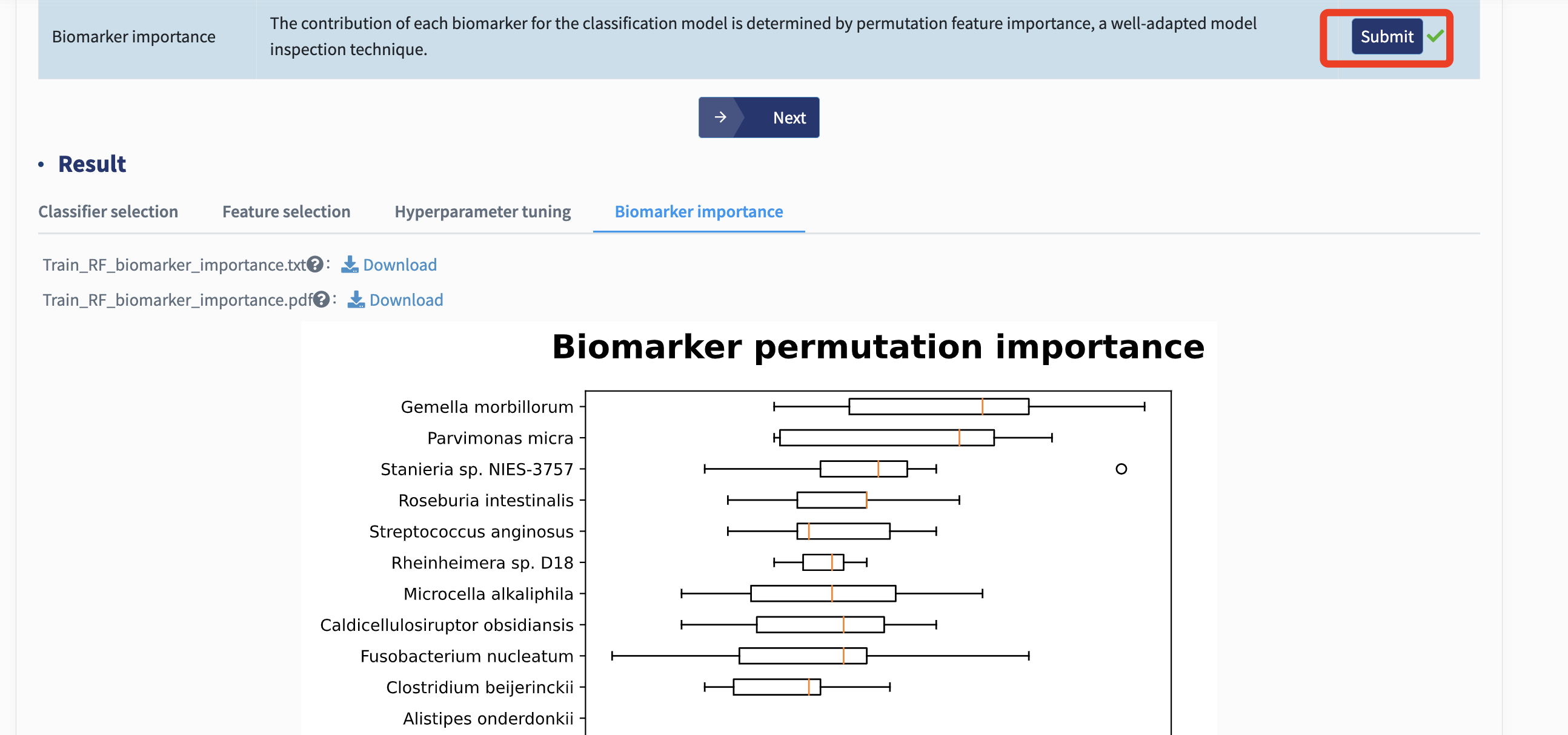
Biomarker importance: The contribution of each biomarker for the best-performing classification model could assist in determining candidate targets for potential interventional practice. Here, xMarkerFinder adopts permutation feature importance, a model inspection technique implemented in scikit-learn. In detail, the decrease of the model AUC is calculated when a single biomarker’s value is randomly shuffled. Therefore, a feature would be defined as important if shuffling its values increases the model error, as the model heavily relies on it.
Model validation
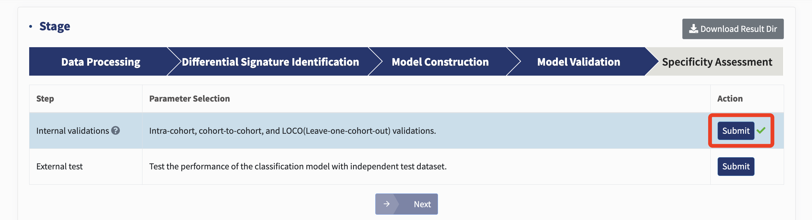
Internal validations: xMarkerFinder assesses candidate biomarkers’ robustness and generalizability at different level within the training dataset, including intra-cohort, cohort-to-cohort, and Leave-one-cohort-out (LOCO) validations.
The intra-cohort validation constructs stratified five-fold cross-validation classification models using profiles of individual cohorts. The performance metrics are calculated against each intra-cohort model, ascertaining that established candidate biomarkers are capable not only in merged cross-cohort discovery dataset but also in individual cohorts.
For cohort-to-cohort transfer, classification model is fit with the profile of one cohort and validated on each profile of the remaining cohorts, respectively. Cohort-to-cohort transfer ensures that models trained on one cohort are applicable on any of the other cohorts.
For LOCO validation, one cohort is ruled out for test, and all other cohorts are pooled together to train the classification model. Both cohort-to-cohort transfer and LOCO validation assess the generalizability of candidate biomarkers in distinct cohorts and could be seen as a simulation of predicting disease-positive samples in a newly established cohort.
Just click Submit!
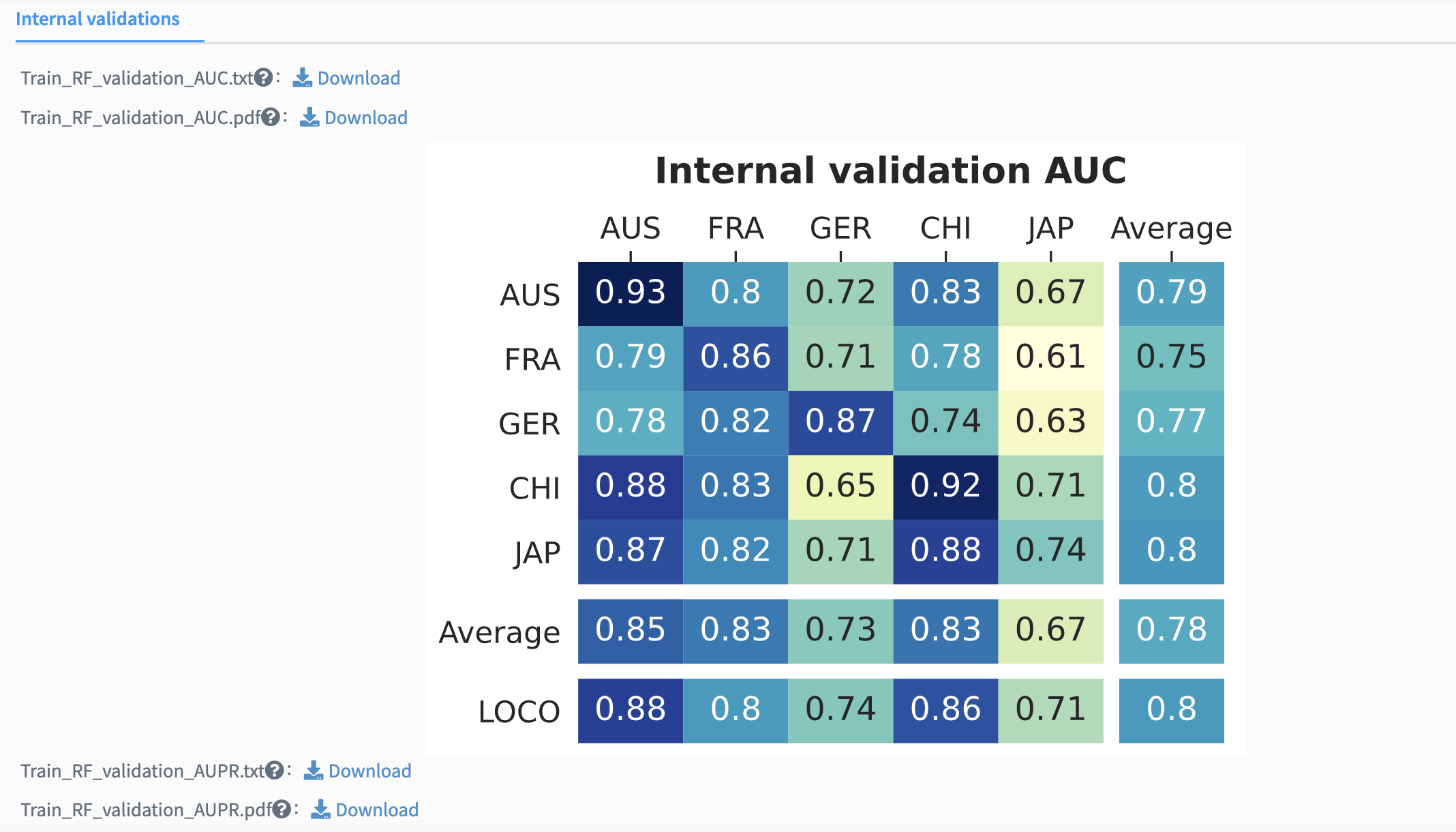
The internal validation results are reported by several model inspection metrics mentioned above. The figures are cross-prediction matrices of the classification model built with candidate biomarkers. Values on the diagonal refer to the average values of stratified five-fold cross-validation within profiles of each cohort. Off-diagonal values refer to the values obtained by training the classifier on the profile of the corresponding row and applying it to the profile of the corresponding column. The LOCO row refers to the performances obtained by training the model using all but the profile of the corresponding column and applying it to the profile of the corresponding column.
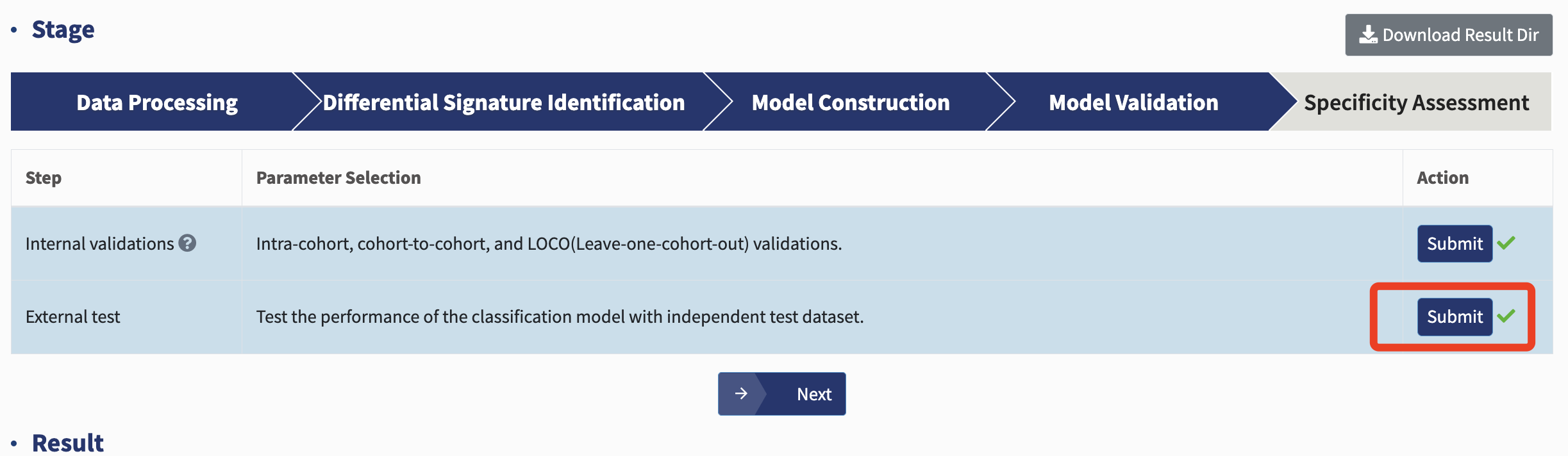
External test: The independent test of the classification model and identified candidate biomarkers is to test their performance with independent test dataset not involved in any discovery steps mentioned above, which ensures their potential applicability in future prospective settings. The best-performing classification model (with the candidate biomarkers and optimal hyperparameters) is used to predict the disease or trait type of the external test dataset, and similarly, multiple performance metrics are employed. Just hit Submit!
Just hit Submit!
Specificity assessment
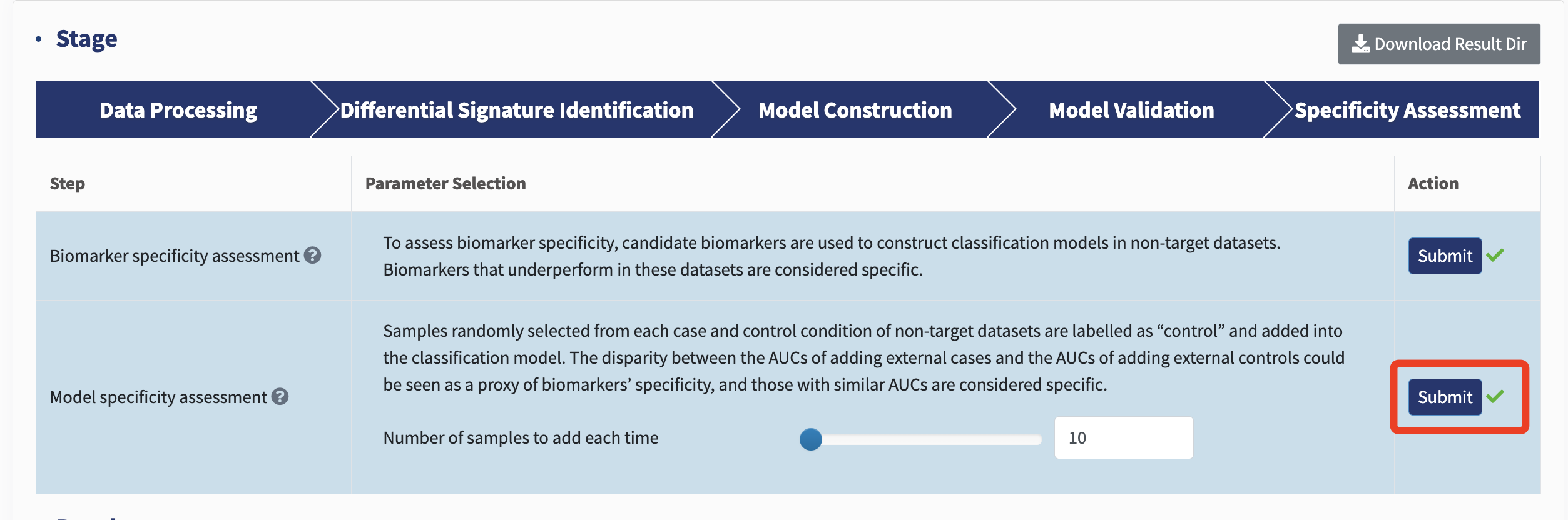
Biomarker specificity assessment: To assess biomarker specificity, candidate biomarkers are used to construct classification models in non-target datasets. Biomarkers that underperform in these datasets are considered specific.
Just hit Submit!
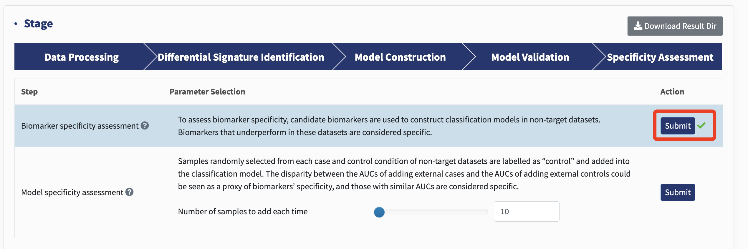
Model specificity assessment: To assess model specificity, xMarkerFinder employs a sophisticated strategy where samples randomly selected from each case and control condition of non-target datasets are labelled as “control” and added into the classification model, and the variations of corresponding AUCs are calculated. The disparity between the AUCs of adding external cases and the AUCs of adding external controls could be seen as a proxy of model specificity, and similar AUCs in non-target datasets signify a model’s specificity.
Users should specify the number of samples to add each time, and click Submit!
Up to this point, you've successfully completed all the analyses! Well done!
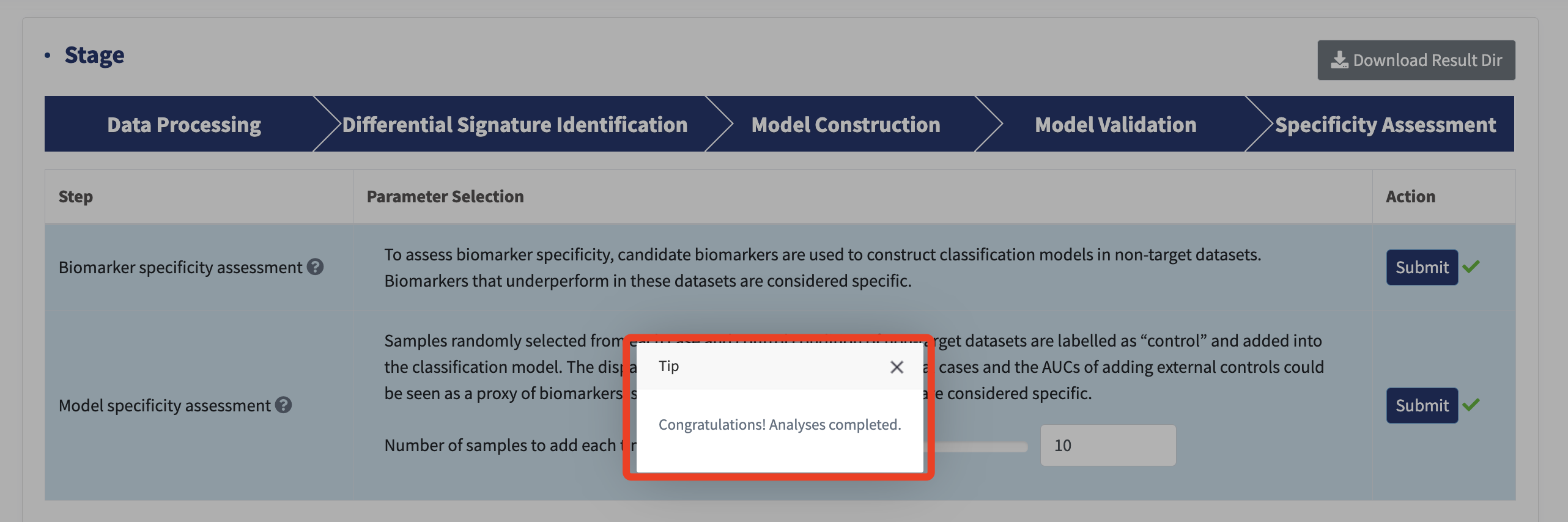
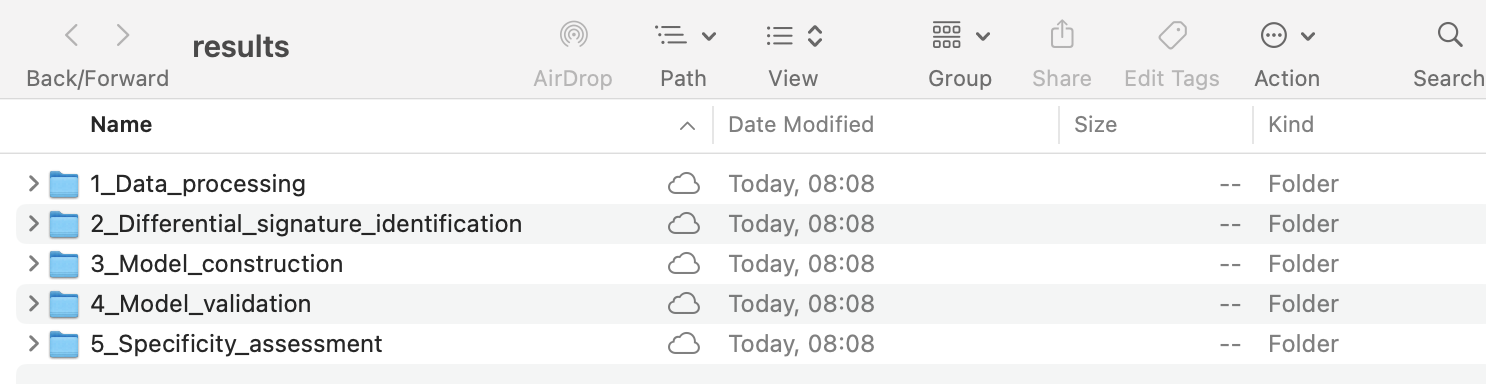
You can download all the results by clicking Download Result Dir
Downstream analysis: Biomarker interpretation
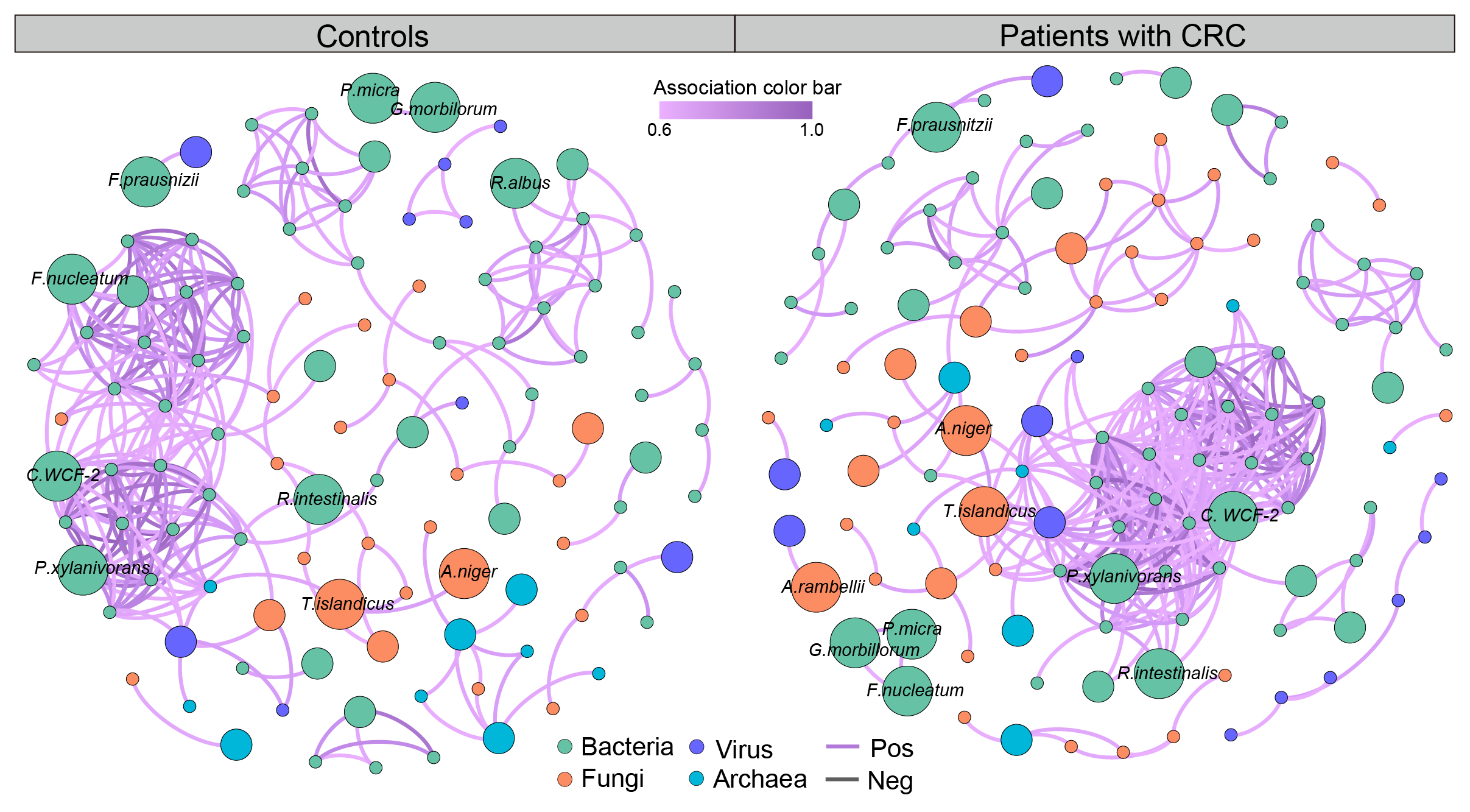
Following the identification and validation of biomarkers from cross-cohort datasets, we further suggest exploring downstream analyses, including biomarker importance, microbial co-occurrence network, and multi-omics correlation, among others.
To enhance user experience, we have incorporated the biomarker importance in the Model construction module on our website (see above). Further, we recommend users to utilize SparCC for the microbial co-occurrence network, and HAllA for multi-omics correlation. See some example results!
We're excited to announce that these features will be incorporated in our upcoming updates. Stay tuned!
In addition to the detailed step-to-step analysis, we’ve also introduced a one-click option for a seamless user experience. Simply select the One-click option and press Submit!
All the steps, along with their respective parameters, are displayed. Users can select each one of them (for more details, please see above) and click the Submit button for a smooth analysis. Kindly wait a moment for the final results!